Guide

This guide covers how the wrapper relates to the underlying Python datasets library, the "julia" format and the transform pipeline, array orientation and working with images, and how to feed a dataset into a Julia data loader — including process-parallel (num_workers) loading that scales past CPython's GIL.

The examples below build small datasets in memory with the Dataset constructor (which accepts a Dict or NamedTuple of columns) so that they are self-contained and reproducible. In practice you will usually obtain a dataset from the Hub with load_dataset, e.g. load_dataset("ylecun/mnist", split="train"); everything shown here applies equally to those datasets.

Loading datasets

load_dataset forwards all its arguments to the Python datasets.load_dataset function. What it returns depends on the split argument:

• without split, you get a DatasetDict (a dictionary of splits), e.g. load_dataset("nyu-mll/glue", "sst2");
• with a split, you get a single Dataset, e.g. load_dataset("nyu-mll/glue", "sst2", split="train").

A DatasetDict is an AbstractDict{String, Dataset}, so keys, values, haskey, get, and iteration all work as expected:

julia> train = Dataset((; label=[1, 0, 1, 0]));

julia> test = Dataset((; label=[1, 1]));

julia> dd = DatasetDict("train" => train, "test" => test)
DatasetDict({
    train: Dataset({
        features: ['label'],
        num_rows: 4
    })
    test: Dataset({
        features: ['label'],
        num_rows: 2
    })
})

julia> collect(keys(dd))
2-element Vector{String}:
 "train"
 "test"

julia> dd["train"]
Dataset({
    features: ['label'],
    num_rows: 4
})

A Dataset supports 1-based indexing, length, firstindex/lastindex (so ds[begin] and ds[end] work), and iteration over observations:

julia> ds = Dataset((; label=[5, 0, 4]));

julia> length(ds)
3

julia> ds[begin]
Dict{String, Int64} with 1 entry:
  "label" => 5

julia> ds[end]
Dict{String, Int64} with 1 entry:
  "label" => 4

julia> [obs for obs in ds]      # iteration yields one observation at a time
3-element Vector{Dict{String, Int64}}:
 Dict("label" => 5)
 Dict("label" => 0)
 Dict("label" => 4)

Indexing with a single integer returns one observation; indexing with a range or vector returns a batch, represented as a dictionary mapping each column name to a vector of values (see below).

Method forwarding

Any method or property of the wrapped Python object is available directly on the Julia wrapper. Method calls are forwarded to Python, and their results are converted back with py2jl. This means the whole datasets API is usable without a dedicated Julia binding for each method:

julia> ds = Dataset((; label=[0, 1, 2, 3]));

julia> ds.select(0:1)                       # keep the first two rows
Dataset({
    features: ['label'],
    num_rows: 2
})

julia> ds.train_test_split(test_size=0.5, seed=42)
DatasetDict({
    train: Dataset({
        features: ['label'],
        num_rows: 2
    })
    test: Dataset({
        features: ['label'],
        num_rows: 2
    })
})

Keyword arguments are forwarded as Python keyword arguments, so calls like train_test_split(test_size=0.5) and shuffle(seed=0) behave exactly as in Python.

Inspecting the schema: features and labels

Every dataset carries a schema describing each column's type. ds.features returns it as a Features view — an AbstractDict from column name to feature type — so you can inspect dtypes and, crucially, decode integer class labels. Indexing a column yields its feature: a Value for a scalar column (carrying an Arrow dtype), a ClassLabel for an encoded label, and so on.

julia> ds = Dataset((; text=["good", "bad", "good"], label=["pos", "neg", "pos"]));

julia> ds.features
{'text': Value('string'), 'label': Value('string')}

julia> ds.features["text"]
Value('string')

The most useful leaf is ClassLabel, which maps integer class ids to names. Turn a string column into one with the forwarded class_encode_column, then read the mapping straight off the feature with Pythonic method chaining (.names, .int2str, .str2int):

julia> ds = Dataset((; label=["pos", "neg", "pos"]));

julia> ds = ds.class_encode_column("label");   # string column -> ClassLabel (names sorted)

julia> cl = ds.features["label"]
ClassLabel(names=['neg', 'pos'])

julia> cl.names
2-element Vector{String}:
 "neg"
 "pos"

julia> cl.int2str(0)            # 0-based class id -> name (no index offset)
"neg"

julia> cl.str2int("pos")
1

julia> ds["label"]              # the stored ids are 0-based data, not 1-based indices
3-element HuggingFaceDatasets.Column{Int64}:
 1
 0
 1

For the common "from a dataset and column name" case there are also public (unexported) Julian shortcuts — class_names, int2str, and str2int — that look up the column's ClassLabel for you (and error clearly if it isn't one):

julia> ds = Dataset((; label=["pos", "neg", "pos"]));

julia> ds = ds.class_encode_column("label");

julia> class_names(ds, "label")
2-element Vector{String}:
 "neg"
 "pos"

julia> int2str(ds, "label", [0, 1, 1])   # decode a batch of ids in one call
3-element Vector{String}:
 "neg"
 "pos"
 "pos"

Reach these as HuggingFaceDatasets.class_names etc., or bring them into scope with using HuggingFaceDatasets: class_names, int2str, str2int. To construct a schema from Julia — e.g. to pass as a features= argument — build the wrapper types (also public but unexported: HuggingFaceDatasets.ClassLabel(names=["neg", "pos"]), HuggingFaceDatasets.Value("int64")) and hand them back to Python with jl2py.

The "julia" format and transforms

Datasets are returned in the "julia" format by default, so indexing yields native Julia values. This format mirrors datasets' own set_format/with_format mechanism and adds an extra Julia-side transform.

Setting a format

with_format returns a copy of the dataset with a given format; set_format! mutates it in place; reset_format! restores the default "julia" format. Passing nothing strips all formatting and hands back raw Python.

julia> ds = Dataset((; label=[5, 0, 4]));   # "julia" format by default

julia> ds[1]
Dict{String, Int64} with 1 entry:
  "label" => 5

julia> ds[1:3]                          # a batch: each column becomes a vector
Dict{String, Vector{Int64}} with 1 entry:
  "label" => [5, 0, 4]

julia> ds["label"]                      # a whole column: a lazy `Column` view
3-element HuggingFaceDatasets.Column{Int64}:
 5
 0
 4

julia> set_format!(ds, nothing);        # strip formatting: raw Python observations

julia> ds[1]
Python: {'label': 5}

Indexing by column name returns a lazy Column: it behaves like a vector (indexing, slicing, iteration, broadcasting) but converts elements only on access, so the whole column is never materialized at once. Call collect to get a plain Vector.

The special "julia" format is backed by datasets' numpy format and sets the Julia transform to py2jl, which recursively converts Python containers (lists, tuples, dicts, sets) and numpy arrays into native Julia values, copylessly when possible. Because the numpy format decodes array and image cells to numeric arrays, an image column comes back as a raw array rather than a colorview (see Working with images). Any other format string (e.g. "numpy", "torch", "pandas") is forwarded to the underlying Python set_format, and nothing clears the format entirely.

Custom Julia transforms

Beyond the format, you can attach an arbitrary Julia function that runs when indexing, with with_jltransform / set_jltransform!. The transform receives the raw Python batch, so convert it with py2jl first if you want to work with Julia types:

julia> ds = Dataset((; x=[1, 2, 3]));

julia> ds = with_jltransform(ds) do batch
           b = py2jl(batch)          # convert the Python batch to Julia types first
           b["x"] .* 10
       end;

julia> ds[1]
10

julia> ds[1:3]
3-element Vector{Int64}:
 10
 20
 30

The transform is always applied to a batch, even for a single-integer index: ds[1] is treated as ds[1:1] from the transform's point of view, and the single observation is then extracted.

Note that the format and the custom transform share the same slot: setting the "julia" format installs py2jl as the transform, and with_jltransform then replaces it — which is why the transform above calls py2jl itself. For layering additional per-batch processing on top of the "julia" format, prefer MLUtils.mapobs (see below), as in the perf/flux_mnist/flux_mnist.jl script.

The order of operations when you index is:

1. the Python format transform (if any) is applied by datasets;
2. the Julia transform runs on the resulting Python batch (for the "julia" format this is py2jl; otherwise your own function);
3. for single-integer indexing, one observation is extracted from the batch.

with_format/with_jltransform return a shallow copy that shares the underlying Arrow data with the original but has an independent format, so setting a format or transform on the copy does not affect the original.

Transforming with map and filter

map and filter are the core datasets verbs for building a new dataset from an existing one. The overloads map(f, ds) / filter(f, ds) bridge the callback for you: each example (or batch, with batched=true) is converted with py2jl before f sees it, and f's Julia return value is converted back to Python with jl2py (the write-path dual of py2jl). You can therefore write a pure-Julia transform while still getting datasets' batching, caching, and multiprocessing:

julia> ds = Dataset((; label=[5, 0, 4]));

julia> ds2 = map(x -> Dict("label" => x["label"] .+ 100), ds; batched=true);

julia> ds2[1:3]["label"]
3-element Vector{Int64}:
 105
 100
 104

julia> ds3 = filter(x -> x["label"] > 2, ds);   # keep rows with label > 2

julia> ds3[:]["label"]
2-element Vector{Int64}:
 5
 4

The property-style calls ds.map(f) / ds.filter(f) are equivalent to map(f, ds) / filter(f, ds) — they route to these same overloads, so the callback still sees Julia values. A DatasetDict behaves the same way: map(f, dd) / dd.map(f) and filter(f, dd) / dd.filter(f) apply f per example across every split (note this makes filter(f, dd) filter examples, not split entries).

A few things to note:

• Batched or not. Without batched=true the callback sees one example at a time (a Dict of scalar values, or whatever py2jl returns); with batched=true it sees a batch (a Dict mapping each column to a vector). Return the same shape: a scalar (map) / Bool (filter) per example, or a vector per column / Vector{Bool} when batched.

• Keyword arguments such as batched, num_proc, and remove_columns are forwarded to the Python method, so multiprocessing and caching work as usual.

• Format is preserved. The returned Dataset inherits the parent's "julia" format (or any custom jltransform), so ds2 above is still "julia"-formatted and a chained pipeline like map(f, dsj) |> ... keeps returning Julia values.

• Raw Python callbacks. To hand map/filter a callback written in "PythonCall dialect" (receiving raw Py rows/batches, pyconvert in, pylist/pydict out), reach for the underlying Python method with ds.py.map(...) / ds.py.filter(...):

  julia> ds.py.map(x -> pydict(label=pylist([pyconvert(Int, l) + 100 for l in x["label"]])),
                   batched=true);      # written against the Python API

Array orientation

Under the "julia" format (backed by datasets' numpy format) an array-valued column decodes to a real N-D numeric array rather than a nested Vector{Vector}, and a range index stacks the rows along the last axis into a (dims…, N) tensor — observation axis last, matching the MLUtils convention:

julia> ds = Dataset((; x = [[1 2 3; 4 5 6], [7 8 9; 10 11 12]]));

julia> ds[1]["x"]                     # one observation: a real 2×3 matrix
2×3 Matrix{Int64}:
 1  2  3
 4  5  6

julia> ds[1:2]["x"]                   # a batch stacks along the last axis
2×3×2 Array{Int64, 3}:
[:, :, 1] =
 1  2  3
 4  5  6

[:, :, 2] =
  7   8   9
 10  11  12

To recover the Python orientation of a single array, reverse the axes with permutedims:

julia> a = numpy2jl(jl2numpy([1 2 3; 4 5 6]));   # a Julia array, transposed vs. numpy

julia> size(a)
(2, 3)

julia> size(permutedims(a, reverse(1:ndims(a))))
(3, 2)

The reverse conversion jl2numpy is symmetric: it shares memory through the buffer protocol and reverses the axes, so numpy2jl(jl2numpy(x)) == x holds and writes propagate in both directions.

Working with images

An Image feature (datasets.Image) is decoded to a numeric array by the numpy format before py2jl sees it, so under the "julia" format an image column is a raw numeric array, not an ImageCore colorview. Combined with the axis reversal above:

• a grayscale (H, W) image becomes a (W, H) UInt8 matrix;
• a color (H, W, C) image becomes a (C, W, H) UInt8 array (channel axis first);
• a fixed-size image column stacks on a range index (to (W, H, N) / (C, W, H, N)), while a ragged (variable-size) column falls back to a Vector of per-row arrays.

That raw layout is what you want for feeding a model (see Data Loaders and the MNIST example), but to look at an image you turn it back into a colorview and undo the transpose with permutedims. Two small helpers cover the common cases:

using HuggingFaceDatasets, ImageCore

# grayscale: (W, H) UInt8  ->  (H, W) Matrix{Gray{N0f8}}
to_gray(a) = permutedims(colorview(Gray, reinterpret(N0f8, a)))

# color: (C, W, H) UInt8   ->  (H, W) Matrix{RGB{N0f8}}
to_rgb(a)  = permutedims(colorview(RGB,  reinterpret(N0f8, a)))

reinterpret(N0f8, a) reads the raw UInt8 bytes as normalized [0, 1] fixed-point values (no copy), colorview wraps the leading axis into Gray/RGB pixels, and permutedims swaps the spatial axes back to the original (H, W) orientation. Rendering the first ten MNIST test digits as a mosaic:

julia> using HuggingFaceDatasets, ImageCore, MosaicViews

julia> ds = load_dataset("ylecun/mnist", split="test");   # "julia" format by default

julia> digits = [to_gray(ds[i]["image"]) for i in 1:10];

julia> mosaicview(cat(digits...; dims=3); nrow=2, npad=1, fillvalue=Gray(1), rowmajor=true)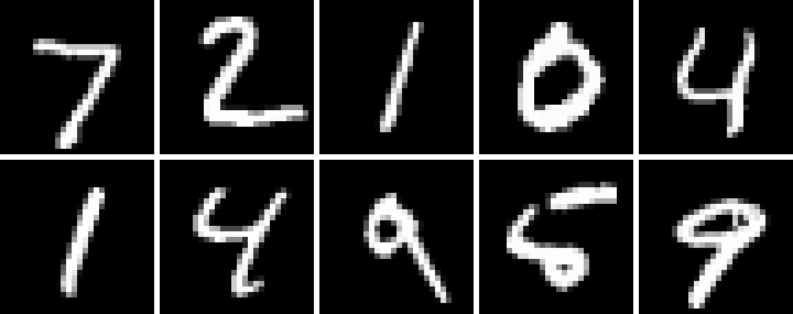

In VS Code, a Pluto/Jupyter notebook, or any ImageInTerminal-enabled REPL such an image renders inline. To write it to disk, add FileIO (with a backend such as ImageIO) and save it:

julia> using FileIO

julia> save("digit.png", to_gray(ds[1]["image"]))

The same to_rgb helper handles color datasets (e.g. to_rgb(ds[1]["img"]) on CIFAR-10), and it round-trips exactly: the recovered array is pixel-for-pixel identical to the image datasets decodes on the Python side.

Integration with MLUtils

A Dataset implements the length/getindex interface expected by MLUtils.jl, so numobs, getobs, and mapobs work directly:

julia> using MLUtils

julia> ds = Dataset((; x=[1, 2, 3, 4]));

julia> numobs(ds)
4

julia> getobs(ds, 2)
Dict{String, Int64} with 1 entry:
  "x" => 2

julia> mapped = mapobs(batch -> batch["x"] .* 10, ds);   # lazily transform observations

julia> getobs(mapped, 1:4)
4-element Vector{Int64}:
 10
 20
 30
 40

Because of this, a Dataset can be handed straight to a data loader — see below.

Data Loaders

A Dataset is a valid MLUtils data container, so you can hand one straight to MLUtils.DataLoader (re-exported by Flux as Flux.DataLoader), including through a mapobs/ObsView transform. The loader's own options are covered in the MLUtils Data Loaders guide; the notes below are specific to a Dataset.

Iterating batches

Each batch is the dataset's own "julia"-format batch: the columns for the batch's rows, stacked and keyed by name (numeric array columns stack into an N-D array with the observation axis last). Small, self-contained example:

julia> loader = DataLoader(Dataset((; x=1:6, y=10:10:60)); batchsize=2);

julia> batch = first(loader);

julia> batch["x"], batch["y"]
([1, 2], [10, 20])

Most training loops want (input, target) pairs rather than a Dict, so wrap the dataset in a mapobs that reshapes each observation; the loader then collates the tuples column-wise into an (inputs, targets) batch you can destructure with for (x, y) in loader:

julia> reshape_obs(o) = (o["x"] * 100, o["y"]);   # per-observation: Dict -> (input, target)

julia> loader = DataLoader(mapobs(reshape_obs, Dataset((; x=1:6, y=10:10:60))); batchsize=2);

julia> first(loader)
([100, 200], [10, 20])

Against the Hub, the same shapes hold — swap the in-memory Dataset for a load_dataset:

julia> using MLUtils

julia> ds = load_dataset("ylecun/mnist", split="train");   # "julia" format by default

julia> loader = DataLoader(ds; batchsize=128, shuffle=true);

julia> batch = first(loader);   # batch["image"] is (28, 28, 128), batch["label"] is length-128

Materializing vs. reading on the fly

For small datasets you can materialize into memory up front with [:] (faster per epoch, no decoding during iteration); otherwise the loader reads on the fly, keeping memory flat:

julia> materialized = DataLoader(ds[:]; batchsize=128, shuffle=true);   # whole dataset in RAM

julia> on_the_fly  = DataLoader(ds; batchsize=128, shuffle=true);       # decode per batch

Layer a per-batch transform with mapobs; with [:] on the mapped dataset the transform runs once up front, without it the transform runs per batch during iteration:

julia> mnist_transform(o) = (Float32.(o["image"]) ./ 255, o["label"]);

julia> train = mapobs(mnist_transform, ds);

julia> loader = DataLoader(train[:]; batchsize=128, shuffle=true);   # or drop [:] for on-the-fly

Parallel loading (num_workers)

Reading on the fly calls into CPython, and CPython's global interpreter lock (GIL) serializes those reads, so thread-based parallel=true gives ~1× on a Dataset. Use num_workers=N instead (needs MLUtils ≥ 0.4.11): it spreads getobs over N worker processes, each with its own interpreter and GIL, so loading scales past the GIL:

julia> loader = DataLoader(ds; batchsize=128, num_workers=4);   # 4 worker processes

julia> for batch in loader
           # ... training step ...
       end

This works because a Dataset serializes by reference to its on-disk Arrow files (an in-memory dataset is first materialized to a temporary Arrow file, announced with an @info), so if you set a jltransform it must be serializable. It composes with a mapobs/ObsView wrapper at any nesting — DataLoader(mapobs(f, ds); num_workers=4) runs f on the workers. Batches may arrive out of input order across workers; combine with shuffle=true (or don't rely on order). Worker processes are launched on demand under the current --project; call MLUtils.close_dataloader_pool() to tear them down. Process parallelism only pays off when getobs is the bottleneck (large images, heavy decode) — for cheap observations the IPC overhead can make it slower than serial. See the MLUtils guide for the mechanics and tradeoffs.

A complete example — mapobs transform, num_workers, and a training loop, benchmarked against PyTorch — lives in perf/flux_mnist/.